Review: Conditional independence
Two random variables X and Y are conditionally independent given a third variable Z if:
p(X, Y \mid Z) = p(X \mid Z) p(Y \mid Z) \tag{4.1}
Equivalently, this means that once we know Z, learning about X tells us nothing additional about Y, and vice versa:
p(X \mid Y, Z) = p(X \mid Z) \quad \text{and} \quad p(Y \mid X, Z) = p(Y \mid Z) \tag{4.2}
We write this as X \perp Y \mid Z (read as “X is independent of Y given Z”).
Conditional independence in graphical models
In Lecture 1, we discussed how graphical models can represent conditional independence relationships among random variables. To make this exhaustive, we’ll consider all possible configurations of three variables connected by two edges. There are four basic graphical model structures, termed v-structures, involving two dependencies among three variables X, Y, and Z:
(a) Indirect causal effect: X \to Z \to Y. Here, Z mediates the relationship between X and Y, and so once we condition on the mediator Z, X and Y become independent, i.e., X \perp Y \mid Z.
(b) Indirect evidential effect: Y \to Z \to X This is the reverse of pattern (a), where Y influences X through Z. The conditional independence relationship is the same, i.e., X \perp Y \mid Z.
(c) Common cause: X \leftarrow Z \to Y. Here, Z is a common cause of both X and Y. Again, X \perp Y \mid Z. Once we condition on the common cause Z, the correlation between X and Y disappears.
(d) Common effect: X \to Z \leftarrow Y. This is the trickiest pattern. Here, Z is caused by both X and Y. In this case, X \perp Y (unconditionally), but X \not\perp Y \mid Z. Conditioning on the common effect Z creates dependence between X and Y. This is sometimes called “explaining away.”
These patterns form the building blocks for understanding more complex probabilistic models. In particular, we will rely on a test called the d-separation test that allows us to determine conditional independence relationships in arbitrary graphical models by breaking them down into these basic patterns.
Next, in state space models, we’ll see how these relationships help us understand the flow of information through time and the conditional independence assumptions that make efficient inference possible.
Hidden Markov models
So far, our modeling of time series has focused on ARMA models. In this lecture, we will introduce a different paradigm for modeling time series, hidden Markov models and linear dynamical systems, which are both examplse of state space models. State space models are a class of probabilistic models that use latent variables to capture the underlying state of a system that evolves over time. These models are particularly useful for modeling time series data where the observations are noisy or incomplete.
Markov models build off of the Markov assumption we introduced in the first lecture:
\begin{align} P\left(X_{1}, X_{2}, \ldots X_{T}\right) &= P\left(X_{1}\right) P\left(X_{2} \mid X_{1}\right) \ldots P\left(X_{T} \mid X_{T-1}\right) \tag{4.3} \end{align}
As we mentioned in the first lecture, we can generalize this assumption to include the k previous random variables for a k^{\text {th }} order Markov model. At the graphical level we depict this model as follows: :::
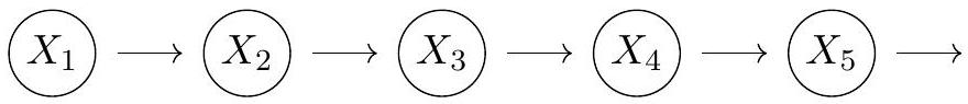
A Markov model of order 1.
While the Markov assumption makes factorizing our joint distribution much easier, it also limits the long-term dependencies we can encode in the data. If we observe X_{t}, then X_{t+1: T} becomes independent of X_{1: t-1}. Ideally, we would have a model that can be specified with a small number of parameters but is not limited in its dependencies by the Markov assumption. To achieve this, we introduce latent variables Z_{t} to pair with our observed stochastic process X_{t}. We can add these latent variables to our Markov model and call the resulting model a hidden Markov model (HMM)1. The figure below shows a graphical model of an HMM of order 1.
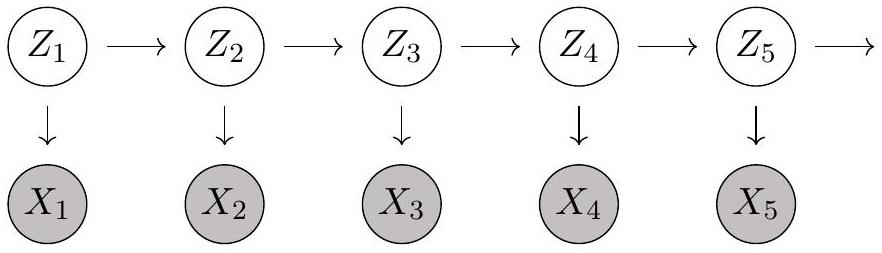
A hidden Markov model of order 1 where the X_t have been observed.
We also will want to move away from dimensionality of one. In fact, the dimensionality of the latent space and the observation space need not be the same. With that in mind, we will start referring to our latent space variables as \boldsymbol{z}_{t} and our observed variables as \boldsymbol{x}_{t}. There are two relevant probabilities from which we will construct all of our equations. These are:
Transition probability distribution function: p\left(z_{t+1} \mid z_{t}\right)
Observation probability distribution function: p\left(x_{t} \mid z_{t}\right)
What are some reasons this may be a better way to model our stochastic process?
Conditional independence properties
Before we dive into a specific case of the HMM, let’s write down a few conditional independence properties given by our model.
The data is d-separated by the latent space observations:
\begin{align} p\left(\boldsymbol{x}_{1: T} \mid \boldsymbol{z}_{t}\right) & =p\left(\boldsymbol{x}_{1: t} \mid \boldsymbol{z}_{t}\right) p\left(\boldsymbol{x}_{t+1: T} \mid \boldsymbol{z}_{t}\right) \tag{4.4}\\ p\left(\boldsymbol{x}_{1: t-1} \mid \boldsymbol{x}_{t}, \boldsymbol{z}_{t}\right) & =p\left(\boldsymbol{x}_{1: t-1} \mid \boldsymbol{z}_{t}\right) \tag{4.5}\\ p\left(\boldsymbol{x}_{t+2: T} \mid \boldsymbol{x}_{t+1}, \boldsymbol{z}_{t+1}\right) & =p\left(\boldsymbol{x}_{t+2: T} \mid \boldsymbol{z}_{t+1}\right) \tag{4.6}\\ p\left(\boldsymbol{x}_{1: T} \mid \boldsymbol{z}_{t-1}, \boldsymbol{z}_{t}\right) & =p\left(\boldsymbol{x}_{1: t-1} \mid \boldsymbol{z}_{t-1}\right) p\left(\boldsymbol{x}_{t} \mid \boldsymbol{z}_{t}\right) p\left(\boldsymbol{x}_{t+1: T} \mid \boldsymbol{z}_{t}\right) \tag{4.7} \end{align}
The future / past latent space is independent from the past / future data given the past / future latent space:
\begin{align} p\left(\boldsymbol{x}_{1: t} \mid \boldsymbol{z}_{t}, \boldsymbol{z}_{t+1}\right) & =p\left(\boldsymbol{x}_{1: t} \mid \boldsymbol{z}_{t}\right) \tag{4.8}\\ p\left(\boldsymbol{x}_{t+1: T} \mid \boldsymbol{z}_{t}, \boldsymbol{z}_{t+1}\right) & =p\left(\boldsymbol{x}_{t+1: T} \mid \boldsymbol{z}_{t+1}\right) \tag{4.9} \end{align}
Given the current latent state, future prediction becomes independent of the data:
\begin{align} p\left(\boldsymbol{x}_{T+1} \mid \boldsymbol{z}_{T}, \boldsymbol{x}_{1: T}\right) & =p\left(\boldsymbol{x}_{T+1} \mid \boldsymbol{z}_{T}\right) \tag{4.10}\\ p\left(\boldsymbol{z}_{T+1} \mid \boldsymbol{z}_{T}, \boldsymbol{x}_{1: T}\right) & =p\left(\boldsymbol{z}_{T+1} \mid \boldsymbol{z}_{T}\right) \tag{4.11} \end{align}
We will take advantage of a few of these as we move forward, but they can all be derived using the graphical model for our HMM. What we will be interested in calculating is the distribution of our latent space variables given our observations. We can write this as:
\begin{align} p\left(\boldsymbol{z}_{t} \mid \boldsymbol{x}_{1: T}\right) & =\frac{p\left(\boldsymbol{x}_{1: T} \mid \boldsymbol{z}_{t}\right) p\left(\boldsymbol{z}_{t}\right)}{p\left(\boldsymbol{x}_{1: T}\right)} \tag{4.12}\\ & =\frac{p\left(\boldsymbol{x}_{1: t} \mid \boldsymbol{z}_{t}\right) p\left(\boldsymbol{x}_{t+1: T} \mid \boldsymbol{z}_{t}\right) p\left(\boldsymbol{z}_{t}\right)}{p\left(\boldsymbol{x}_{1: T}\right)} \tag{4.13}\\ & =\frac{p\left(\boldsymbol{x}_{1: t}, \boldsymbol{z}_{t}\right) p\left(\boldsymbol{x}_{t+1: T} \mid \boldsymbol{z}_{t}\right)}{p\left(\boldsymbol{x}_{1: T}\right)} \tag{4.14}\\ & =\frac{\alpha\left(\boldsymbol{z}_{t}\right) \beta\left(\boldsymbol{z}_{t}\right)}{p\left(\boldsymbol{x}_{1: T}\right)} \tag{4.15} \end{align}
where we have set \alpha\left(\boldsymbol{z}_{t}\right)=p\left(\boldsymbol{x}_{1: t}, \boldsymbol{z}_{t}\right) and \beta\left(\boldsymbol{z}_{t}\right)=p\left(\boldsymbol{x}_{t+1: T} \mid \boldsymbol{z}_{t}\right) for notational convenience.
Forward and backward recursions
This framing is useful because we can calculate both \alpha and \beta recursively. Let’s start with \alpha and apply some of our conditional independence properties:
\begin{align} \alpha\left(\boldsymbol{z}_{t}\right) & =p\left(\boldsymbol{x}_{1: t}, \boldsymbol{z}_{t}\right) \tag{4.16}\\ & =p\left(\boldsymbol{x}_{1: t} \mid \boldsymbol{z}_{t}\right) p\left(\boldsymbol{z}_{t}\right) \tag{4.17}\\ & =p\left(\boldsymbol{x}_{t} \mid \boldsymbol{z}_{t}\right) p\left(\boldsymbol{x}_{1: t-1} \mid \boldsymbol{z}_{t}\right) p\left(\boldsymbol{z}_{t}\right) \tag{4.18}\\ & =p\left(\boldsymbol{x}_{t} \mid \boldsymbol{z}_{t}\right) p\left(\boldsymbol{x}_{1: t-1}, \boldsymbol{z}_{t}\right) \tag{4.19}\\ & =p\left(\boldsymbol{x}_{t} \mid \boldsymbol{z}_{t}\right) \int p\left(\boldsymbol{x}_{1: t-1}, \boldsymbol{z}_{t-1}, \boldsymbol{z}_{t}\right) d \boldsymbol{z}_{t-1} \tag{4.20}\\ & =p\left(\boldsymbol{x}_{t} \mid \boldsymbol{z}_{t}\right) \int p\left(\boldsymbol{x}_{1: t-1}, \boldsymbol{z}_{t} \mid \boldsymbol{z}_{t-1}\right) p\left(\boldsymbol{z}_{t-1}\right) d \boldsymbol{z}_{t-1} \tag{4.21}\\ & =p\left(\boldsymbol{x}_{t} \mid \boldsymbol{z}_{t}\right) \int p\left(\boldsymbol{x}_{1: t-1} \mid \boldsymbol{z}_{t-1}\right) p\left(\boldsymbol{z}_{t} \mid \boldsymbol{z}_{t-1}\right) p\left(\boldsymbol{z}_{t-1}\right) d \boldsymbol{z}_{t-1} \tag{4.22}\\ & =p\left(\boldsymbol{x}_{t} \mid \boldsymbol{z}_{t}\right) \int p\left(\boldsymbol{x}_{1: t-1}, \boldsymbol{z}_{t-1}\right) p\left(\boldsymbol{z}_{t} \mid \boldsymbol{z}_{t-1}\right) d \boldsymbol{z}_{t-1} \tag{4.23}\\ & =p\left(\boldsymbol{x}_{t} \mid \boldsymbol{z}_{t}\right) \int \alpha\left(\boldsymbol{z}_{t-1}\right) p\left(\boldsymbol{z}_{t} \mid \boldsymbol{z}_{t-1}\right) d \boldsymbol{z}_{t-1} \tag{4.24} \end{align}
As we will show for a linear dynamical system (LDS) below, this recursive relation will make our calculation easier. We can think of this as the forward pass of our estimation. We can do the same for \beta to get our backward pass:
\begin{align} \beta\left(\boldsymbol{z}_{t}\right) & =p\left(\boldsymbol{x}_{t+1: T} \mid \boldsymbol{z}_{t}\right) \tag{4.25}\\ & =\int p\left(\boldsymbol{x}_{t+1: T}, \boldsymbol{z}_{t+1} \mid \boldsymbol{z}_{t}\right) d \boldsymbol{z}_{t+1} \tag{4.26}\\ & =\int p\left(\boldsymbol{x}_{t+1: T} \mid \boldsymbol{z}_{t+1}\right) p\left(\boldsymbol{z}_{t+1} \mid \boldsymbol{z}_{t}\right) d \boldsymbol{z}_{t+1} \tag{4.27}\\ & =\int p\left(\boldsymbol{x}_{t+1} \mid \boldsymbol{z}_{t+1}\right) p\left(\boldsymbol{x}_{t+2: T} \mid \boldsymbol{z}_{t+1}\right) p\left(\boldsymbol{z}_{t+1} \mid \boldsymbol{z}_{t}\right) d \boldsymbol{z}_{t+1} \tag{4.28}\\ & =\int \beta\left(\boldsymbol{z}_{t+1}\right) p\left(\boldsymbol{x}_{t+1} \mid \boldsymbol{z}_{t+1}\right) p\left(\boldsymbol{z}_{t+1} \mid \boldsymbol{z}_{t}\right) d \boldsymbol{z}_{t+1} \tag{4.29} \end{align}
This gives us all the terms in the numerator for Equation 4.15, with the remaining term serving as a normalization for our posterior on the latent variables.
Prediction of future observations
The final property we want to derive is how to predict future observations given our current set of observations:
\begin{align} p\left(\boldsymbol{x}_{T+1} \mid \boldsymbol{x}_{1: T}\right) & =\int p\left(\boldsymbol{x}_{T+1}, \boldsymbol{z}_{T+1} \mid \boldsymbol{x}_{1: T}\right) d \boldsymbol{z}_{T+1} \tag{4.30}\\ & =\int p\left(\boldsymbol{x}_{T+1} \mid \boldsymbol{z}_{T+1}\right) p\left(\boldsymbol{z}_{T+1} \mid \boldsymbol{x}_{1: T}\right) d \boldsymbol{z}_{T+1} \tag{4.31}\\ & =\int p\left(\boldsymbol{x}_{T+1} \mid \boldsymbol{z}_{T+1}\right) \int p\left(\boldsymbol{z}_{T+1}, \boldsymbol{z}_{T} \mid \boldsymbol{x}_{1: T}\right) d \boldsymbol{z}_{T+1} d \boldsymbol{z}_{T} \tag{4.32}\\ & =\int p\left(\boldsymbol{x}_{T+1} \mid \boldsymbol{z}_{T+1}\right) \int p\left(\boldsymbol{z}_{T+1}, \boldsymbol{z}_{T} \mid \boldsymbol{x}_{1: T}\right) d \boldsymbol{z}_{T+1} d \boldsymbol{z}_{T} \tag{4.33}\\ & =\int p\left(\boldsymbol{x}_{T+1} \mid \boldsymbol{z}_{T+1}\right) \notag \\ &\quad\quad \int p\left(\boldsymbol{z}_{T+1} \mid \boldsymbol{z}_{T}\right) p\left(\boldsymbol{z}_{T} \mid \boldsymbol{x}_{1: T}\right) d \boldsymbol{z}_{T+1} d \boldsymbol{z}_{T} \tag{4.34}\\ & =\frac{1}{p\left(\boldsymbol{x}_{1: T}\right)} \int p\left(\boldsymbol{x}_{T+1} \mid \boldsymbol{z}_{T+1}\right) \notag \\ &\quad\quad\quad \int p\left(\boldsymbol{z}_{T+1} \mid \boldsymbol{z}_{T}\right) \alpha\left(\boldsymbol{z}_{T}\right) d \boldsymbol{z}_{T+1} d \boldsymbol{z}_{T} \tag{4.35} \end{align}
We can extend this to predicting the next state given the observed data:
p\left(\boldsymbol{z}_{T+1} \mid \boldsymbol{x}_{1: T}\right)=\frac{1}{p\left(\boldsymbol{x}_{1: T}\right)} \int p\left(\boldsymbol{z}_{T+1} \mid \boldsymbol{z}_{T}\right) \alpha\left(\boldsymbol{z}_{T}\right) d \boldsymbol{z}_{T} \tag{4.36}
We will circle back to these concepts once we’ve introduced our specific case.